Prerequisites

This article assumes that you’re at least somewhat familiar with the concept of full-waveform inversion (FWI). For an overview of what FWI is, check out this article.

What is the Adjoint Method?

One of the most important parts of full-waveform inversion (FWI) is how we are able to figure out which part of our model we should be tweaking. However, getting this sort of “map” of which parts of our medium we should adjust to lead to an improvement of our data fit is a non-trivial task.

These types of maps correspond to the gradients of the misfit function and are often colloquially referred to as “gradients”.

The term “misfit function” refers to some technique we use to compare how similar our observed and our synthetically generated data are to each other (if you’re not sure what I mean by this, check out this article). If we think intuitively of what the gradient of something represents, it’d tell us in which direction we need to move something in order for the value of that thing to increase (or decrease if we reverse the direction of the gradient). The gradient of the misfit function, thus, essentially tells us how we should change the material properties of our medium so that the misfits decrease (ie. the differences between the observed and synthetically generated data).

The technique we use to get the gradients of the misfit function is known as the adjoint method:

The adjoint method is a clever mathematical trick that lets us come up with the gradients of the misfit function by comparing how similar two wavefield are.

While the physical meaning behind these gradients is somewhat intuitive, the process of how we get these gradients can be a little tricky to wrap our head around. Let’s break down each of the individual steps we perform within the adjoint method:

1. Calculating the forward wavefield.
2. Compare the synthetically generated measurements we just created to the observed data to get the adjoint sources.
3. Re-inject the adjoint sources backwards in time to get the adjoint wavefield.
4. Correlate the forward wavefield and the adjoint wavefield together.

Note: The examples demonstrated below are based on work presented at the 2022 IEEE International Ultrasonics Symposium (IUS)¹.

1. Calculate the Forward Wavefield

As was discussed in the FWI article previously, we need to have some starting model from which we begin the inversion. What we want to do first is take this starting model and fire an ultrasound source to see how the ultrasound waves propagate through the starting model. There are two things we want to do here:

1. Record the ultrasound signals within this forward simulation at the same positions where we have measured data for.
2. Save the entire forward wavefield in memory for later.

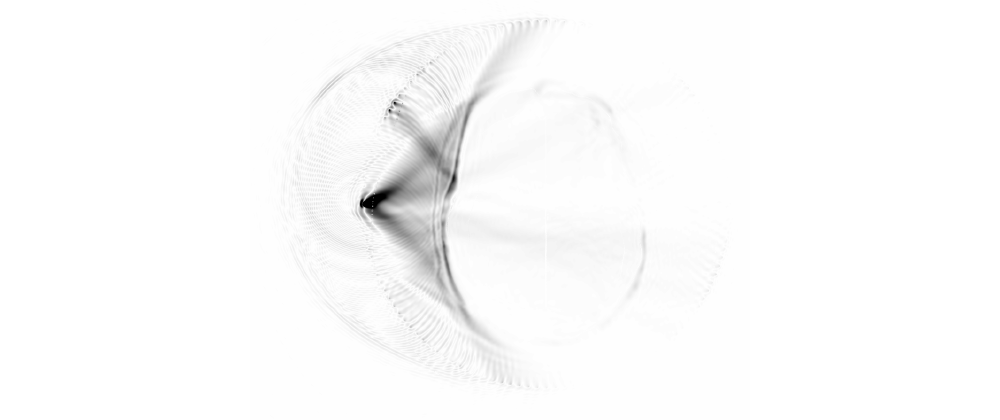
If we consider a brain imaging application where we assume our starting model consists of the geometry of the skull, our forward wavefield would look something like this:

In the above example, the halo of points surrounding the skull represent the receiver locations.

2. Get the Adjoint Sources

Next, we want to compare the observed signals to the synthetically generated ones we just created. There are a bunch of different types of metrics or so-called misfit functions we could use to compare the two signals — the choice in misfit function generally depends on the application. A few common misfit functions include:

• \(l^2\) norm
• Cross-correlation
• Time-frequency
• Optimal transport

The \(l^2\) norm is generally the most intuitive one to understand so we’ll use that as an example. This essentially just compares how different the amplitudes are between two signals. The result of this calculation is the adjoint sources which we’ll use to get the adjoint wavefield in the next step. Since we do this calculation for each receiver position, we have one unique adjoint source for each receiver location.

3. Calculate the Adjoint Wavefield

Now that we have the adjoint sources, we can calculate the adjoint wavefield. To do this, we take the adjoint sources we calculated in the previous step and re-inject them at the receiver positions backwards in time.

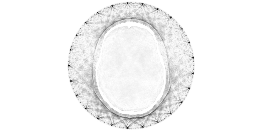
This process is best illustrated by an example, so let’s see what the adjoint wavefield would look like for the previous forward modelling example:

Notice that the time axis for the above simulation was flipped (ie. it ran backwards in time). We would save this adjoint wavefield in memory so that we can correlate it with the forward wavefield in the next (and final) step of the adjoint method.

4. Correlate the Forward and Adjoint Wavefields

The final step to the adjoint method involves correlating together the forward and adjoint wavefields to get the gradients of the misfit function.

What this means in practice is that if we were to “playback” the forward/adjoint simulations, we’d have a bunch of time slices where we saved the wavefield output. What we want to do as we “playback” the wavefield simulations we calculated in steps 1. and 3. involves first multiplying together each time slice and then sum all of the time slices together.

Here’s what this process would look like:

This gradient shows us where we should perturb our material properties (for that specific source position) to lead to an improvement in data fit.

---

Some Important Nuances

While the adjoint method is a very powerful way for us to get the gradients, there are a few caveats which we’ve glossed over in the previous sections but which are important to be aware of.

Computational Cost

The computational cost of using the adjoint method is usually dominated by the two wave simulations we need to perform:

• Forward wavefield
• Adjoint wavefield

For many practical applications, these computational costs are so high that we are forced to run these wave simulations on high-performance computing clusters. For example, in my research we use the Piz Daint supercomputer from the Swiss National Supercomputing Centre, which is one of the most powerful supercomputers in Europe. As computational hardware continues to improve in the future, being able to perform these computations on a single high-perfornace workstation will likely become feasible.

Gradients for Each Source Positions

Related to the high computational cost of performing the wave simulations using the adjoint method is the impact on the number of sources within our simulation setup.

As we saw within the previous example, we calculated the gradient for a single source position. However, to illuminate more of the tissue of the patient we’d often want to fire several ultrasound sources in sequence. The consequence of this is that we need to derive a gradient for each source position in our ultrasound device.

This means that the computational cost scales linearly with the number of sources in our ultrasound device. There are some tricks such as “source encoding” which involves firing several ultrasound sources within the same simulation so that we can reduce the number of wave simulations we need to perform. However, this can often introduce what’s known as “crosstalk” between the different measurements which makes the resulting inverse problem more difficult to solve as a result.

Memory Requirements and Checkpointing

One of the simplifications we made to the previous example is that we saved the wavefield outputs in memory. However, doing this for many practical applications in 3D could potentially consume several petabytes of data (a petabyte is a million gigabytes).

To get around this, what we can do instead is save what are known as “checkpoints” of our forward wavefield. This involves saving a bunch of snapshots of the wavefield so that we can reduce the memory overhead of having to store the forward wavefield for when we perform our subsequent adjoint run.

For example, let’s say our simulation would have 1000 time steps we’d have to compute the wave equation for. We could then save every 10th time slice so that we’d have 100 checkpoints saved instead of saving all 1000 time slices in memory.

Due to reasons which I won’t get into here, using checkpointing will increase the overall computational cost somewhat since we need to eventually re-calculate these time slices which we threw away once we perform our adjoint simulation. However, checkpointing is a really powerful tool that lets us drastically reduce the memory requirements of using the adjoint method.

---

What the Underlying Math Looks Like

For a deeper theoretical look at the adjoint method I’d highly recommend chapter 8 of this book:

Fichtner, A. (2011). Full Seismic Waveform Modelling and Inversion. Springer-Verlag. https://doi.org/10.1007/978-3-642-15807-0

If you’ve made it this far, you may be curious about what the underlying math looks like for the adjoint method. Let’s take a brief look at some of the key parts of the adjoint method.

Some Preliminaries

Something which you’ll often see with these types of derivations is something like:

Consider a position vector \(\mathbf{x} \in \Omega \subset \mathbb{R}^2\) for the times \(t \in T\).

All this means is that here we have some sort of physical domain in 2D which we call \(\Omega\) where we can describe it’s spatial coordinates using \(\mathbf{x}\). Similarly, we’re interested in looking at some times \(t\) within some time interval \(T\).

The Forward Problem

$$ \mathbf{L}(\mathbf{u}, \mathbf{m}) = \mathbf{f} $$

where :

• \(\mathbf{L}\) is a symbolic forward operator that represents the wave equation,
• \(\mathbf{u}\) is the observable quantity (so something like the pressure or the displacement of the wavefield),
• \(\mathbf{m}\) are the model parameters (such as the material properties of the tissues we are trying to image), and
• \(\mathbf{f}\) is a source term (the energy that would be injected into the system from the ultrasound sources).

This equation is what’s used to solve the forward problem.

The Gradient of the Misfit Function

We want to use some sort of misfit function \(\chi (\mathbf{m})\) to describe how similar or different our observed data (the data we’d gather in the lab or in a hospital) to our simulated data (what we calculate when we solve the above forward equation). As mentioned earlier in this article, there are many possible difference metrics which we could use to compare our data with this choice typically being application dependent.

In any case, what we generally want to try and find is the gradient of the misfit function with respect to our model parameters \(\nabla_\mathbf{m} \chi\) as this will tell us how we should tweak our model parameters to lead to a decrease in our misfits. I won’t go through the derivation of the gradient of the misfit function here, but in the end it works out to

$$ \nabla_\mathbf{m} \chi \cdot \delta \mathbf{m} = \int \limits_T \int \limits_\Omega \mathbf{u}^\dagger \cdot \nabla_\mathbf{m} \mathbf{L} (\mathbf{u}) \delta \mathbf{m} \\; \text{d} \mathbf{x}^2 \\; \text{d} t. $$

This equation looks pretty formidable, but it’s actually pretty intuitive to what we discussed with the previous (visual) examples. Let’s break down what each part of this equation represents physically.

The Left-Hand-Side

$$ \textcolor{default}{\nabla_\mathbf{m} \chi \cdot \delta \mathbf{m}} \textcolor{lightgray}{= \int \limits_T \int \limits_\Omega \mathbf{u}^\dagger \cdot \nabla_\mathbf{m} \mathbf{L} (\mathbf{u}) \delta \mathbf{m} \\; \text{d} \mathbf{x}^2 \\; \text{d} t} $$

The gradient of the misfit function is the key thing which we’re trying to find using the adjoint method. Since we’re looking at a directional derivative, this notation means that we want to try and find the gradient of the misfit function with respect to some model parameter \(\mathbf{m}\) in a direction \(\delta \mathbf{m}\).

This model parameter \(\mathbf{m}\) could be something like the density, compressional (P-wave) speed of sound, or shear (S-wave) speed of sound. So let’s say we’d want to find the derivative of the misfit function with respect to the P-wave velocity, we could express this as something like \(\nabla_{v_p} \chi \cdot \delta v_p\).

The Forward Wavefield

$$ \textcolor{lightgray}{\nabla_\mathbf{m} \chi \cdot \delta \mathbf{m} = \int \limits_T \int \limits_\Omega \mathbf{u}^\dagger \cdot} \textcolor{default}{\nabla_\mathbf{m} \mathbf{L} (\mathbf{u}) \delta \mathbf{m}} \textcolor{lightgray}{\\; \text{d} \mathbf{x}^2 \\; \text{d} t} $$

As we discussed previously, the forward operator \(\mathbf{L} (\mathbf{u})\) describes the solution to the wave equation. Therefore, this describes the forward wavefield which propagates through our starting model.

The Adjoint Wavefield

$$ \textcolor{lightgray}{\nabla_\mathbf{m} \chi \cdot \delta \mathbf{m} = \int \limits_T \int \limits_\Omega} \textcolor{default}{\mathbf{u}^\dagger} \textcolor{lightgray}{\cdot \nabla_\mathbf{m} \mathbf{L} (\mathbf{u}) \delta \mathbf{m} \\; \text{d} \mathbf{x}^2 \\; \text{d} t} $$

The adjoint wavefield is denoted by \(\mathbf{u}^\dagger\) (spoken out loud as “u-dagger”). As we saw in the above example, we re-inject our adjoint sources at the receiver positions backwards in time and let the wavefield propagate until the start time (usually time zero) of the simulation. This often has a sort of “focusing effect” where the adjoint wavefield tends to focus at the source position from the forward run.

The Integrals

$$ \textcolor{lightgray}{\nabla_\mathbf{m} \chi \cdot \delta \mathbf{m} =} \textcolor{default}{\int \limits_T \int \limits_\Omega} \textcolor{lightgray}{\mathbf{u}^\dagger \cdot \nabla_\mathbf{m} \mathbf{L} (\mathbf{u}) \delta \mathbf{m}} \textcolor{default}{\\; \text{d} \mathbf{x}^2 \\; \text{d} t} $$

One of the key steps to obtaining the gradient of the misfit function is that we integrate over both space (denoted by \(\Omega\)) and time (denoted by \(T\)).