Full-Waveform Inversion
What is Full-Waveform Inversion?
Full-waveform inversion (commonly referred to as FWI) is conceptually very simple despite the underlying math behind it being relatively complex.
At its most fundamental level, full-waveform inversion is simply a fancy data fitting algorithm.
Using FWI, we can come up with very detailed reconstructions (images) of the interior structure of a medium by fitting the waveforms (or acoustic wiggles) that our acoustic device measures.

Let’s consider an analogous example to first introduce the idea of FWI.
Analogous Example: With Pie!
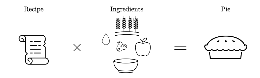
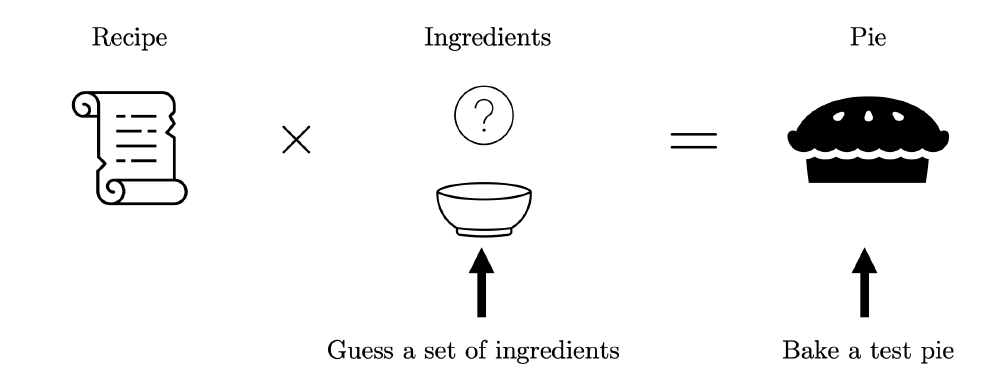
Let’s say our friend bakes us a pie (yes, the food). The process of baking the pie can be described as a forward problem — that is, we take some set of known model parameters (the ingredients of the pie), we apply some known process to it (the recipe), and then we get a tangible result out of it (the baked pie).

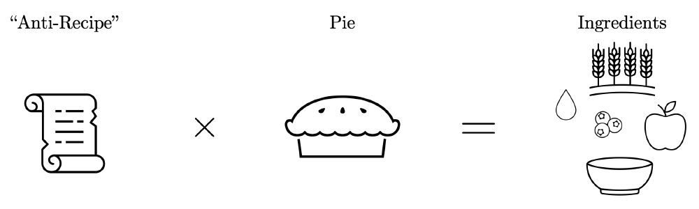
However, let’s say we’d want to take the pie that our friend gave us and we’d want to figure out what ingredients go into making the pie. This could be thought of as the inverse problem where we would take the pie (the observed “data”), we’d then apply an “anti-recipe” to “unbake” the pie, and then get back the raw ingredients. Of course, the idea of “unbaking” the pie is ridiculous — we’d be trying to undo whatever chemical reactions would have occurred during the baking process.

Luckily there’s an intuitive alternate strategy we could take instead. Let’s assume that we’re reasonably skilled bakers, so we know more-or-less how we’d go about baking a pie. In this sense, the recipe would be known to a sufficient degree through some a priori knowledge of the type of system we’re trying to solve. What we could try then is to simply guess a set of ingredients, bake a “test pie” using our approximate recipe, and then check how close our prediction is to the pie that our friend gave us.

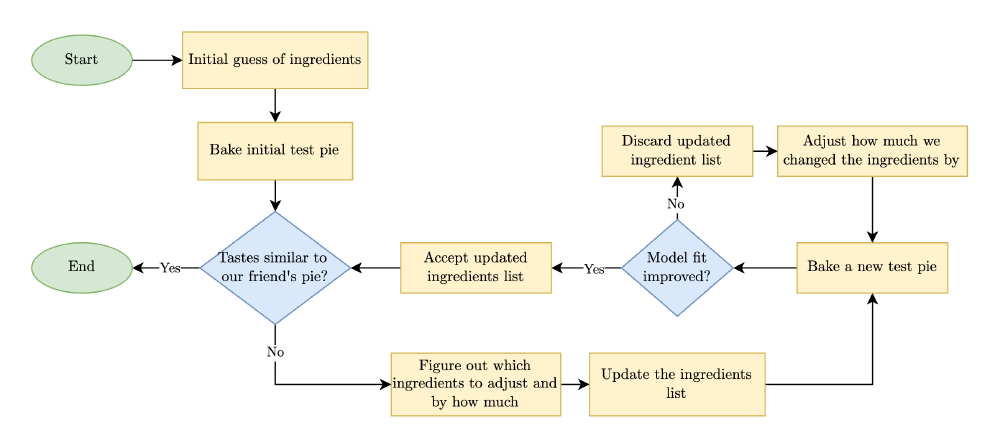
This process of figuring out what ingredients are used to bake our friend’s pie can be thought of as an incremental or “iterative” process. If we bake our first test pie, we can then check and see how close our pie is to the one our friend baked. Using this information, we can adjust our list of ingredients so that our next test pie will (hopefully) be even more similar to our friend’s pie.
There are, of course, several things we need to keep in mind when trying to solve this problem:
- Baking a Test Pie is Expensive
- The ingredients that go into baking a pie are expensive, so we want to try and minimize the number of times that we bake a test pie.
- Inexact Recipe
- Since we don’t know the exact recipe, we may be neglecting some additional complexities (eg. slightly different baking temperatures/times).
- We need our approximate recipe to be “good enough”. What constitutes as being “good enough” is highly problem-dependent.
- Initial Guess
- If our initial guess of the ingredients is poor, we probably won’t be able to adjust the ingredients in any meaningful way to get a pie that is close to our friend’s.
- For example, if our friend baked an apple-blueberry pie but we include tuna fish and capers within our initial guess, it is extremely unlikely that we’ll know what ingredients to adjust since the two pies will be so different from each other.
- Getting the Exact Ingredient List is Unlikely
- It is very unlikely that we’ll be able to recover the exact ingredient list.
- We want to try and get a list of ingredients that is “good enough”.
We can show this pie baking inverse problem as an algorithm similar to the following:

Bringing Things Back to Medical Imaging
While this pie baking example may seem silly at first, there are many close parallels with this and what we perform within FWI. Here are the analogues which we have within medical FWI when compared to the pie example:
| Technical Term | Pie Example | Medical Ultrasound |
|---|---|---|
| Model Parameters | Ingredients | Material properties of the tissues |
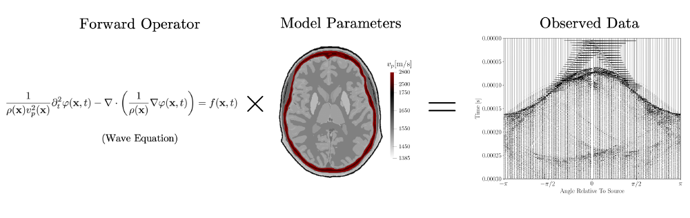
| Forward Operator | Recipe | Wave operator |
| Observed Data | Pie | Ultrasound waveforms |
Putting things in terms of a similar schematic to what we had for the pie example, we can consider the forward problem for the brain imaging problem to be something like the following:

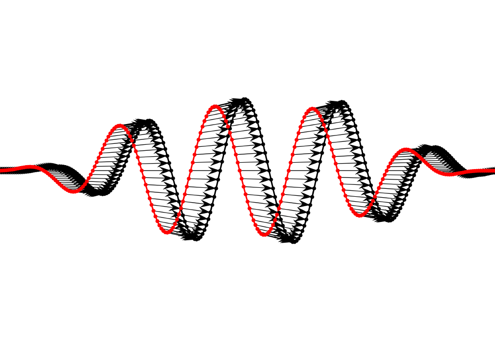
It’s pretty tricky to try and make any meaningful interpretations from the wiggles (also known as waveforms) that make up our observed data. This is why we want to try to solve the inverse problem where we try and find what material properties went into generating these waveform.
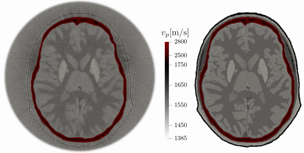
Different tissues throughout the body vary in material properties. For example, material properties of density or speed-of-sound vary greatly between muscle and fat. The consequence of this is that ultrasound waves reflect and refract across these material boundaries. In essence, the model parameters we are trying to recover in medical ultrasound problems consists of an image which shows us what material properties are located where within the tissue. This has a very important implication which is what sets ultrasound computed tomography apart from many other types of medical imaging modalities:
Ultrasound computed tomography creates quantitative images.
This is of great interest as this can serve as a great way to distinguish healthy from cancerous tissue, for example.
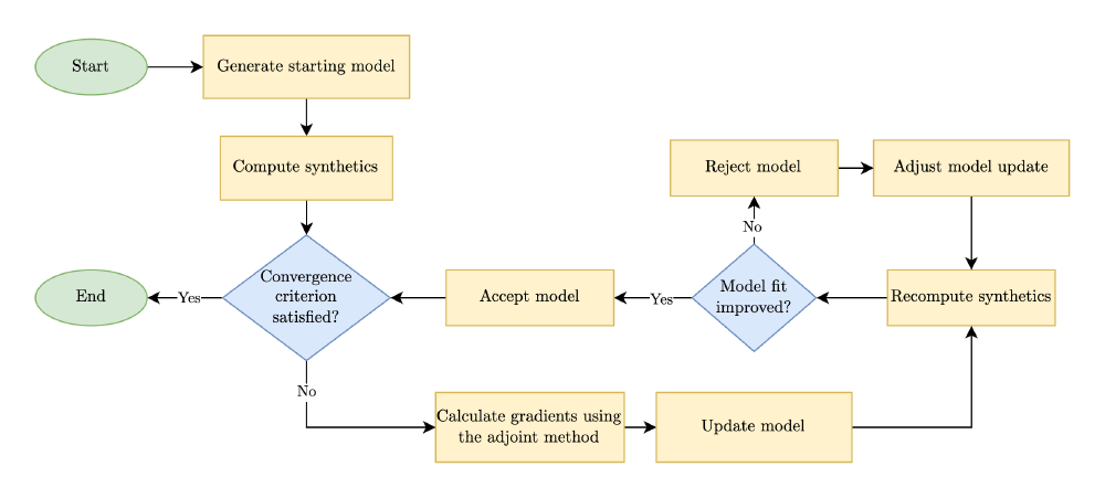
The workflow we use here is remarkably similar to what we previously had for the pie example:
![]()
The process of how we go about getting this reconstructed image is quite similar to what we did in the pie example: we want to try and make an educated guess of what the material properties of the brain tissue are. What we would do with this “guess” of the material properties is that we would run a wave simulation using those material properties where we model how the ultrasound waves move through the brain. We would then record the ultrasound waveforms (ie. the little wiggles from the previous figure) and compare them to the waveforms we recorded in the lab.
This of course assumes that we can perform these wave simulations very accurately so that the physics that we’re modeling is the same (or at least very close) to what’s actually happening in real life.
The Adjoint Method
One of the key steps to performing FWI is a process known as the adjoint method. I won’t go into details on what the adjoint method is here, but in broad terms it’s a very clever mathematical trick that lets us come up with a “map” of how we should adjust the medium we’re trying to image. This is what tells us where and how we should tweak our initial guess of the material properties.
Since this process is quite involved, I’ve written a separate article here which goes over how this technique works.
Practical Example: Brain Imaging
To see an example of how full-waveform inversion can be applied to imaging the human brain, see here.