What is the Finite-Element Method?

There are lots of equations that are incredibly useful in science and engineering that are applied all the time in solving complicated physics problems. Here are a few examples:

• Solid mechanics: Figuring out how stuff deforms when we apply different forces to it. Useful for:
  • Constructing buildings, bridges, tunnels, or dams
  • Designing the structural components of a vehicle
• Fluid dynamics: Studying how fluids interact with other objects. Useful for:
  • Calculating how air moves over anything that needs to be aerodynamic (eg. airplane, F1 car, etc)
  • Designing rocket or airplane engines
• Acoustics: Seeing how sound waves (mechanical waves) reflect and refract as they travel through a material. Useful for:
  • Designing large open spaces like opera or lecture halls
  • Imaging the subsurface when exploring for geothermal energy

What do all of these systems have in common? They’re all really complicated problems because they have:

• Complex geometries
• Lots of different parts, components, and/or materials

All of these types of physics have certain underlying equations that we need to solve to study their behaviour. However, there is usually only a closed-form solution (ie. an equation that we can actually solve) for “special” or simple cases which are usually limited in their usefulness when applied to these more complicated setups.

An example of this from civil engineering is how we are able to easily calculate how a single beam deflects if we apply a load to one end of it. However, we don’t have a single equation that can solve this same type of loading problem if we want to study a complicated bridge that has many beams interacting with each other.

This has a very significant consequence:

We are not able to solve these fundamental equations exactly — we instead need to come up with an approximation which gives us a result that is “good enough”.

These types of math problems are called differential equations and describe how our system changes in space and/or time (in math terms, we would have derivatives in both space and/or time). Since we can’t solve these differential equations exactly for many complicated systems, we often turn to different numerical methods to try and come up with approximations to these equations. Some common numerical approaches to approximate these types of systems include:

• Finite-elements
• Finite-differences
• Boundary-elements

The way that all of these techniques work is by taking our medium and splitting it up into many little pieces. This way, we can approximate the solution to these differential equations over each of these tiny pieces individually. This step of splitting up the domain into many little bite-sized pieces is known as discretizing the domain and the method by which the domain is decomposed into these little pieces is very different for each of these numerical techniques.

Since we use the spectral-element method (a special version of the finite-element method) for solving the wave equation here, we’ll consider how we discretize a medium into finite-element meshes throughout this article.

What Is a Mesh?

In the finite-element method, we split up our medium into a bunch of little pieces or “elements” that (usually) consist of either little triangles or quadrilaterals (deformed squares) in 2D; in 3D these become deformed pyramids (tetrahedra) or cubes (hexahedra). The resulting discretization that we create is known as a mesh.

Why Are Meshes Important?

One of the reasons why the finite-element method is so widely used in engineering applications is because of how well-suited it is for dealing with complex geometries. If we’re clever about how we build our finite-element mesh, we can have the edges of the elements follow the interfaces between two materials exactly, for example.

Accurately resolving the interfaces between two distinct materials can be absolutely critical with describing how our physics behaves across these boundaries.

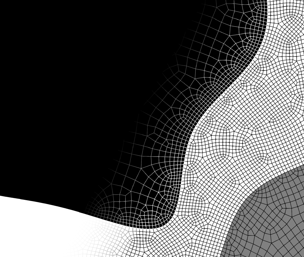
To give an idea as to why this is so important, let’s consider a simple ultrasound simulation where we want to describe how sound waves move from one material to another. Here’s a simple example where we fire an ultrasound source in the middle of three distinct materials:

The spiderweb-like grid represents our finite-element mesh. Here we’ve explicitly meshed the interfaces between the different materials so that we accurately describe how the ultrasound waves would reflect and refract across these interfaces.

That then begs the question: “What would happen if we don’t accurately mesh these interfaces?”

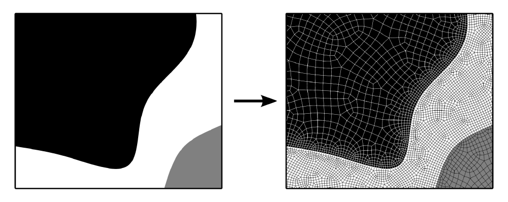
One of the most straight-forward ways of creating such a finite element mesh would be to simply take a rectilinear mesh (a regular grid of rectangular elements) and tack on the material properties we’d want to represent in our medium. This leads to so-called staircasing which occurs when we try representing curved boundaries on a rectilinear grid; the interface appears jagged like stair steps. This can lead to some pretty nasty artifacts once we run our wave simulation as we can see below; the staircased mesh is on the left while the precise mesh is on the right:

As we can see above, the staircased interface (the jagged one on the left) ends up introducing many additional reflections behind the primary reflected and transmitted wavefronts. If we accurately mesh this interface, as on the right side above, we’re able to avoid these additional erroneous reflections altogether.

Tetrahedral vs Hexahedral Meshes

Something you may have noticed in all of the previous examples is that the meshes use quadrilateral elements only; that is, small deformed squares. The reason that we use quadrilateral elements here instead of triangular ones is that the particular type of finite-element method we use here to calculate the wave equation (known as the spectral-element method) benefits significantly by using quadrilateral elements. I won’t get into the nitty-gritty as to why this is, but the important thing is that using quadrilateral elements instead of triangular elements in the spectral-element method can speed up our calculations by a factor of about 100 to 1000 times.

These benefits extend to 3D meshes as well. These quadrilateral and triangular elements are used to construct 2D meshes; the 3D versions of these are called hexahedral and tetrahedral elements, respectively. As with all things in life though, there’s a caveat with using quadrilateral or hexahedral meshes:

Constructing hexahedral (or quadrilateral) meshes is significantly more difficult than constructing tetrahedral (or triangular) meshes.

Constructing Hexahedral Meshes

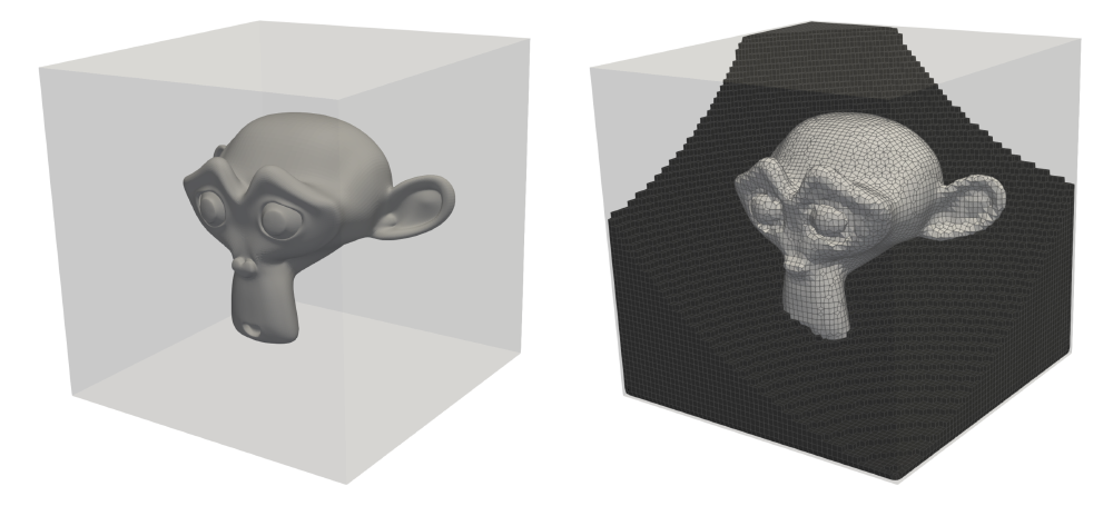
Here’s an example using the Blender monkey known as Suzanne, which is commonly used as a test model in 3D graphics. We can see a comparison between the surface mesh (generated in Blender) and the resulting hexahedral mesh (generated in Coreform Cubit):

These hexahedra essentially fill the entire volume which we want to mesh. As a result, the files used to store these meshes can quickly become extremely large in size.

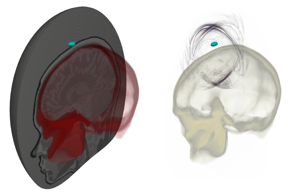
This can, of course, be used for more practical things. Here we’ve constructed an all-hex mesh of the skull which is used for performing an ultrasound simulation. The mesh and the accompanying wavefield can be seen below:

Computational Cost and Numerical Stability

The numerical approximation we use to solve the wave equation is only stable under certain circumstances.

This means that if we violate a certain set of conditions, then the simulation will break and the values we’re trying to calculate will explode to infinity. There’s a criterion known as the CFL criterion (named after the three people that discovered it: Courant-Friedrichs-Lewy) which we can use to figure out what characteristics our simulation needs to have so that the simulation doesn’t break. There are three main parameters that we can use to describe this:

• \(v_\text{min}\): Lowest speed-of-sound in the medium.
• \(\Delta \boldsymbol{x}\): Approximate element size.
• \(\Delta t\): Time step.

such that \(\text{CFL} < 1.0\). This has some pretty significant implications for the overall computational cost:

Making the elements smaller (ie. making the mesh finer) requires us to also reduce the time step to make sure that the simulation remains stable.

Why is this such a big deal? Imagine we have a simulation where we want to model how some sound waves move through a material over the course of 10 seconds. Let’s say for the sake of example that our time step is \(\Delta t = 0.1~\text{s}\). That would mean we would have 100 time steps in our simulation. If we reduce the element size, we’re also required to reduce this time step \(\Delta t\) to make sure that the simulation remains stable.

Let’s say that this adjustment in the element size forces us to reduce the time step to \(\Delta t = 0.025~\text{s}\). Now we suddenly have 400 time steps meaning we’ve increased our computational cost by 4 times because of the increase in the number of time steps alone! Not only do we have more time steps that we need to calculate, but since our mesh is finer, we also have more elements in our mesh that we need to solve the wave equation over.

The moral of the story: Making the discretiation finer is always a double whammy when it comes to the computational cost:

• Finer discretization equals more elements.
• Smaller elements equals more time steps.