Overview

In this article we’ll go through the process of creating a torus knot and then use it for simulating the propagation of an acoustic wavefield.

Here I’m just going to go over the general procedure for how one could go about performing such a simulation. While these techniques can be applied using your choice of software tools, here are the ones I’ve used:

• Blender
  • Initial prototyping and compositing of videos.
• Coreform Cubit
  • Hexahedral mesh generation.
• Salvus
  • Acoustic wave simulation.
• ParaView
  • Visualising and rendering the wavefield.

What is a Torus Knot?

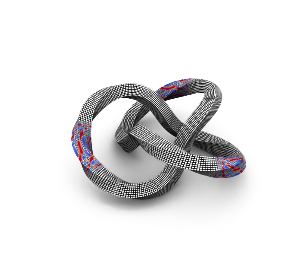
The torus knot is a piece of geometry that looks quite intricate, but is surprisingly easy to construct. It’s essentially a closed loop (i.e. like a doughnut) which is knotted in on itself. Here’s an example of one particular type of torus knot known as the trefoil knot:

The equations that are used to describe each point on a torus knot are:

$$ \begin{aligned} x &= r \cos{(p \, \varphi)} \\ y &= r \sin{(p \, \varphi)} \\ z &= - \sin{(q \, \varphi)} \end{aligned} $$

where \(p\) and \(q\) are some integer values that change the shape of the knot and \(\varphi\) are angles in the range of \(\varphi \in [0, 2\pi)\). The parameter \(r\) can be calculated as

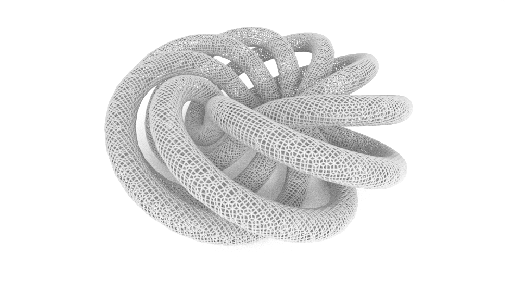
$$ r = \cos{(q \, \varphi)} + 2. $$

Here are a few different examples of torus knots for different choices of \(p\) and \(q\):

For the remainder of this example, we’ll choose \(p = 2\) and \(q = 3\) (the parameters required for creating a trefoil knot) for no particular reason, other than that it looks cool.

Creating the Volume Model

Let’s first begin with constructing the volume geometry in Coreform Cubit. This geometry is what we’ll subsequently use to create a hexahedral mesh, which we can then use for our wave simulation. To start, I’m first going to get the \(x\)-, \(y\)-, and \(z\)-coordinates of the torus knot using the equations above. I’ve chosen the angles \(\varphi\) to be equally spaced (as well as choosing quite a dense sampling of \(\varphi\)) so that the knot looks quite smooth.

I thought it’d look neat to use a square cross section for the torus knot instead of a circular one. We can also quite nicely visualize how the knot twists as it wraps around itself. To achieve that, I placed a plane representing the cross section of the knot at a given point. I then oriented it so that the normal vector of the plane was in-line with the direction from a particular point to the next point along the knot.

There’s a pretty easy way to calculate the rotation angles required to orient the plane correctly. First, we want to get the orientation of the axis about which we want to rotate the plane. This can be obtained by taking the cross product between the normal of the plane and the orientation pointing from the current point in the knot to the next point.

Let’s look at what equations describe these rotations. Let’s treat \(\mathbf{x}_i\) as being the cartesian coordinate for the current point, where \(\mathbf{x}_{i+1}\) would be the coordinate of the next point in the knot. This means that the orientation vector \(\mathbf{d}_i\) is

$$ \mathbf{d}_i = \mathbf{x}_{i+1} - \mathbf{x}_i, $$

since the direction vector from one point to another is just the point at the head of the vector minus the point at the tail of the vector.

We can then get the rotation axis \(\mathbf{r}_i\) by taking the cross product between the normal vector of the plane \(\hat{\mathbf{n}}_i\) and the direction vector \(\mathbf{d}_i\) using

$$ \mathbf{r}_i = \hat{\mathbf{n}}_i \times \mathbf{d}_i. $$$$ \hat{\mathbf{n}}_i \cdot \mathbf{d}_i = \| \hat{\mathbf{n}}_i \| \| \mathbf{d}_i \| \cos{\theta_i}. $$

Re-arranging then for \( \theta_i \), we get

$$ \theta_i = \cos^{-1} \left( \frac{\hat{\mathbf{n}}_i \cdot \mathbf{d}_i}{\| \hat{\mathbf{n}}_i \| \, \| \mathbf{d}_i \|} \right). $$

Once all of the planes have been added, we want to loft between all of the individual planes to turn the planes into volumes. A loft essentially just acts to extrude a volume from one cross section to another.

Here’s what the entire process looks like in Coreform Cubit:

Constructing the Mesh

The geometry created by this sequence of lofts lends itself quite nicely for constructing a high-quality hexahedral mesh, which we can then use for a wave simulation.

The general strategy which we want to follow here is to mesh the cross section of each lofted volume so that we can sweep it from one lofted body to the next. We can repeat this for every subvolume (i.e. each coloured part in the previous animation) to get then a single continuous hexahedral mesh.

Here’s what that looks like:

Here I’ve used a mapped meshing scheme to resolve the individual cross sections, but you could also use something like the paving algorithm in case you’re using a cross section that isn’t a square.

Wave Simulation

Now that we a hexahedral mesh for this torus knot, we can feed this into a spectral-element solver to model the propagation of sound waves along the knot. Here I’ve used the spectral-element solver called Salvus.

Since the relative length of the knot is quite large, we’re going to place a total of three sources in the knot — one in each “arm” of the knot. I didn’t want to just use one source since the waves will have already decreased in amplitude considerably due to geometrical spreading by the time they’d reach the other side of the knot.

Here’s what the resulting simulation looks like for the torus knot:

Even though the overall complexity of this example is “relatively” simple, I think it does quite a nice job at illustrating how complicated the wavefield can become purely due to the geometry of the domain. All of the material properties (speed of sound, density, etc.) throughout the knot are uniform — all of the wave interactions are only due to the curved surface geometry.

This is also where the spectral-element method (and other finite-element methods for that matter) really shine. Since we can mesh these interfaces explicitly, we can achieve remarkable levels of geometric accuracy when we compute a solution to the wave equation.