Prerequisites

This article assumes that you’re at least somewhat familiar with the concept of full-waveform inversion (FWI). For an overview of what FWI is, check out this article.

Imaging the Brain with Ultrasound

There are two main imaging techniques which are widely used to image the human skull/brain: computed tomography (CT) and magnetic resonance imaging (MRI).

While both of these techniques are extremely useful tools for diagnosing various brain related conditions, they both come with some significant drawbacks:

• CT: Exposes the patient to X-rays.
  • This makes CT less well-suited for performing repeated measurements on the same patient for long term monitoring.
• MRI: Cost, long acquisition times, and limited applicability for some patients.
  • The high up-front cost of these scanning devices coupled with their significant operational costs can make MRI prohibitively expensive to use, particularly in places with less robust healthcare systems.
  • The lengthy acquisition times can lead to longer wait-list times for patients given that fewer patients can be scanned within a single day. Furthermore, these lengthy acquisition times can make applying MRI within pediatrics challenging given that the patient is required to lie still for an extended period of time.
  • There are some limitations in the types of patients which can be scanned using MRI. For example, MRI may be an unsuitable modality for patients with metallic implants.

To try and tackle these challenges, my PhD project has been exploring strategies for using ultrasound imaging as an alternative modality for imaging the human brain. This type of imaging is typically referred to as transcranial ultrasound.

Why Can’t Existing Ultrasound Methods Image the Brain?

There are two main reasons why existing ultrasound methods struggle to produce full reconstructions of the brain:

1. Most conventional ultrasound imaging techniques make certain assumptions about the material properties they’re trying to image — namely that the variations in the material properties are relatively limited. However, this assumption quickly breaks down when we try imaging soft tissues that are near bones; the speed-of-sound in bone is about twice as high as that in soft tissue.
2. Accounting for the fluid-solid coupling between soft tissue and bone is tricky; we generally refer to these fluid and solid regions as acoustic or elastic, respectively. When waves travel from a solid to a fluid (or vice versa), we get the conversion between different types of mechanical waves, which considerably complicates the wavefield. Most conventional ultrasound methods can’t account for these coupling effects.

How Can Geophysics Help?

There are two common geophysics problems which share many of the challenges with transcranial ultrasound:

• Subsalt Imaging:
  • This is a common type of imaging target within hydrocarbon exploration.
  • Hydrocarbons tend to get trapped close to these distinct salt layers within the subsurface.
  • The salt layers which one is trying to image close to typically possess a much higher speed-of-sound when compared to the surrounding rock.
  • This material contrast is comparable to what we have to deal with in transcranial ultrasound.
• Core-Mantle Boundary:
  • The boundary between the outer core (fluid) and the mantle (solid) within the deep interior of the Earth is very irregular.
  • When we perform earthquake simulations, we often have these seismic waves travel across these boundaries.
  • We need to have strategies in place to correctly account for the interactions at this fluid-solid boundary.

To try and image these types of domains, an algorithm known as full-waveform inversion is commonly applied within geophysics.

Numerical Example

Note: The example demonstrated below is based on work presented at the 2022 IEEE International Ultrasonics Symposium (IUS)¹.

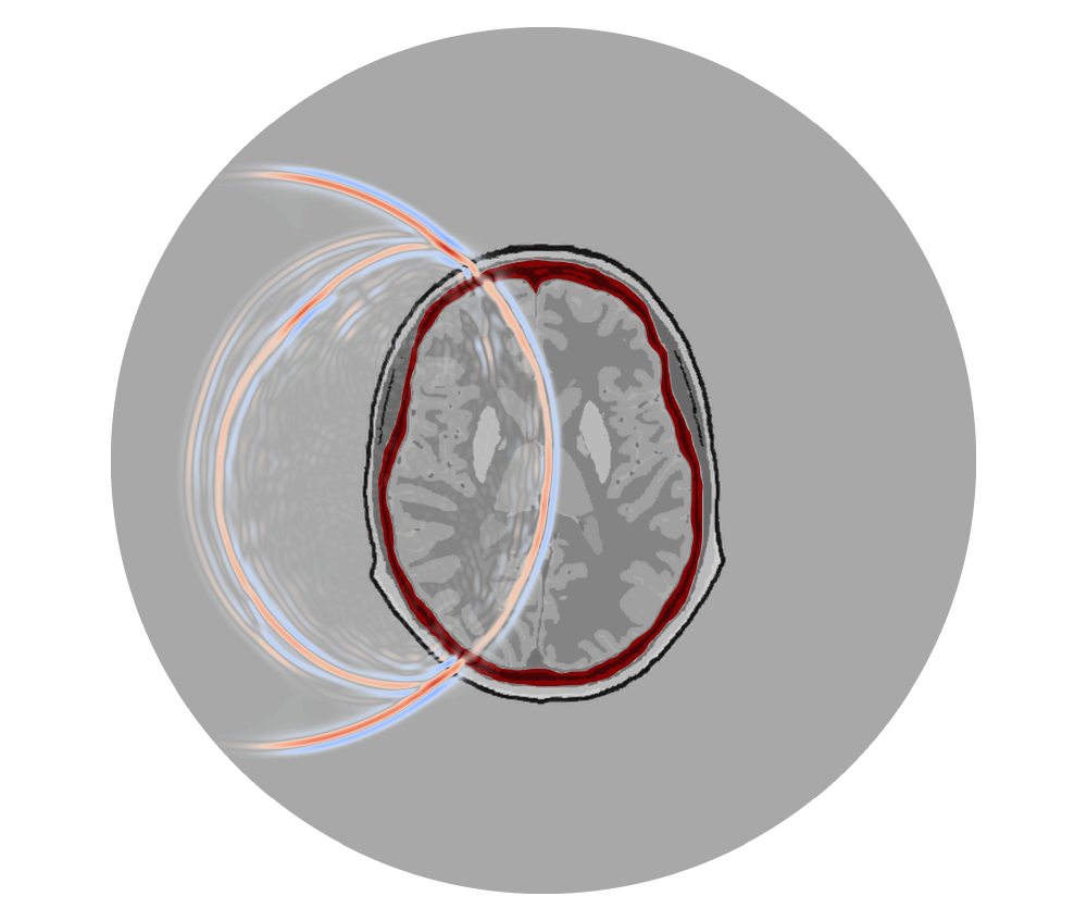
Below is a numerical example which demonstrates the capabilities of FWI for imaging the brain using ultrasound. This type of numerical example is often referred to as in silico, meaning that the “observed” data has been generated using a realistic computer model; the observed data here was not collected in a lab or clinical setting.

Here we start from an initial model where we assume that we know the geometry of the skull and the scalp before beginning the inversion. In this case, we’ve used a process known as reverse time migration (RTM) to figure out the positions of the scalp and skull interfaces. A key step to constructing this initial model involves explicitly meshing the interfaces between the soft tissue and the skull using the techniques discussed here.

The compressional (P-) wave velocity (denoted by \(v_p\)) is inverted for within this example. This material property controls how quickly waves propagate through them and is one of the key inversion parameters within many FWI applications:

There are a number of key parts to this inversion which are discussed below.

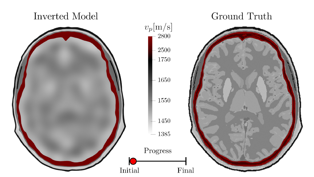
1. Fitting the Longer Wavelength Structures First

As can be seen in this example, the longer wavelength structures are resolved first. This is achieved by using a combination of a few different techniques:

• Low-pass filter the observed data to remove the higher frequencies in the signal.
• Smooth the gradients between model updates.
• Use a large maximum expected time shift within the optimal transport misfit function used for this example. (This acts as a tuning parameter which allows for one to either place a greater emphasis on changes in phase versus changes in amplitude between two signals.)

Combining all of these strategies leads to relatively smooth updates being applied right at the beginning of the inversion.

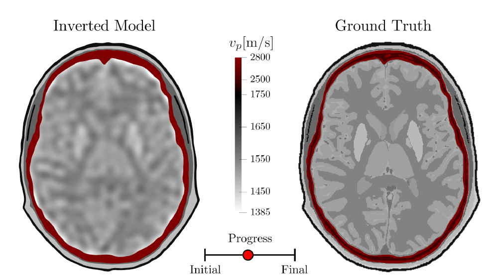
2. Inverting for Finer-Scale Structures

As the inversion continues, the aforementioned inversion parameters are adjusted to help sharpen up the image:

• Higher frequencies are reintroduced into the observed signal.
• The smoothing length used for regularizing the gradients between model updates is reduced.
• Reduce the maximum expected time shift to place a greater emphasis on correcting for changes in amplitude as opposed to changes in phase.

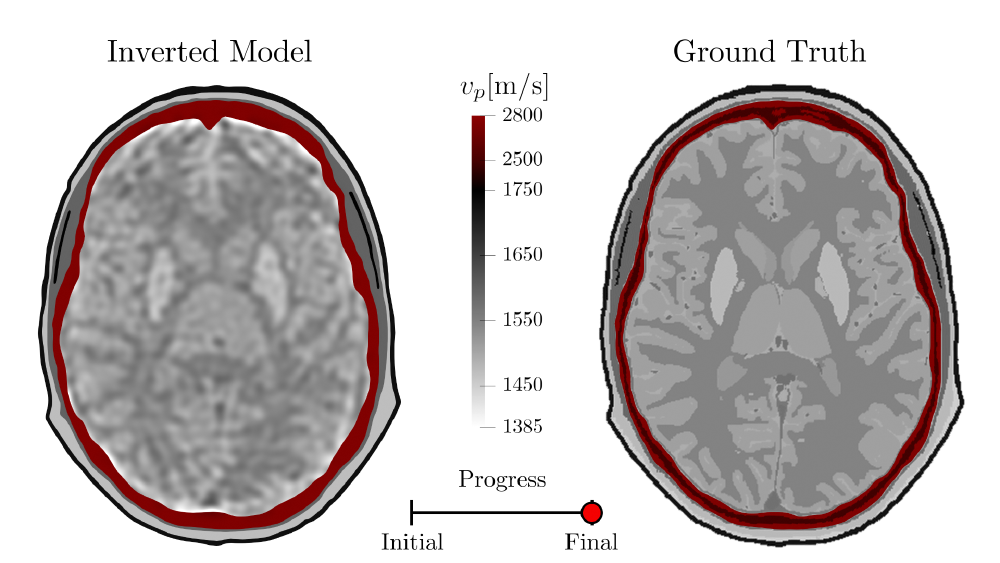
3. Sharpen Up Edges Between Tissues

Finally, the parameters adjusted in step 2. are scaled further such as to sharpen up the interfaces between the different tissues. While this part of the inversion certainly helps to make the features within the brain tissue better defined and easier to interpret, this part of the inversion (usually) doesn’t introduce radical new changes in the overall structure of the reconstruction. Instead, the rough features delineated within the previous steps are further refined.

This last portion of the inversion shows why it is important to resolve the longer wavelength structures within the early stages of the inversion. Using higher frequencies, short smoothing lengths, and small maximum expected time shifts helps to sharpen up the image. However, this fundamentally assumes that we are already in the “vicinity” of where the optimal model is. If we were to immediately to try and resolve these fine-scale features without first resolving the longer wavelength structures first, we’d likely end up with a (physically) unrealistic reconstruction.