How Waves Move Through Materials

Accurately modelling the propagation of sound waves through different materials is vital for fields including:

• Medical ultrasound imaging
• Seismology
• Non-destructive testing

The primary equation of interest for these types of problems is known as the wave equation.

There are many different types of wave equations which describe how mechanical waves move through fluids, solids, or porous materials. One of the simplest versions of the wave equation is the so-called acoustic wave equation, which describes how pressure waves move through fluids. Throughout this article, we’ll only be looking at the acoustic wave equation.

A Simple Example: Uniform Square

Let’s say we set up a loudspeaker in the middle of a square room. If we’d want to avoid having any reverberations off of the walls of the room, we could put foam sound panels on the walls to absorb the sound that’s produced by the loudspeaker. If we play a single burst of sound from the loudspeaker and look at a top-down view of the room, here’s how the sound waves would spread out throughout the room:

In this very simple example we’ve inject a source at the center of a square domain. Here the material properties throughout the entire domain are uniform (homogeneous) which means that the waves don’t reflect or refract throughout the medium. We’ve added absorbing boundaries to the medium so that the waves disappear as they get close to the edges of the square.

The background grid represents the mesh on which we perform the calculations necessary for solving the wave equation. I’ve got a dedicated article here on how we can go about constructing these sorts of meshes.

Heterogeneous Media

Things get a little more interesting once we add heterogeneities within our material. Let’s consider a layered medium where we have three deformed circular layers of differing material properties. Here there are three distinct materials:

• Inner most layer: fastest speed-of-sound
• Middle layer: slowest speed-of-sound
• Outer layer: median speed-of-sound (with no absorbing boundaries)

As we can see, the waves get both reflected and transmitted across the boundaries between the different parts of the medium. In general, the stronger the material contrast, the more energy is reflected back. Similarly, the lower the material contrast, the more of the energy gets transmitted across the boundary.

Practical Example: Brain Imaging

These wave simulations look neat and all, but what are they actually useful for?

One application that I work on in my research is studying how ultrasound waves move through the brain. If we can better understand how the ultrasound waves interact with the soft tissues and the skull, we may be able to develop a technique similar to MRI or CT which let’s us come up with images of the internal structure of the brain.

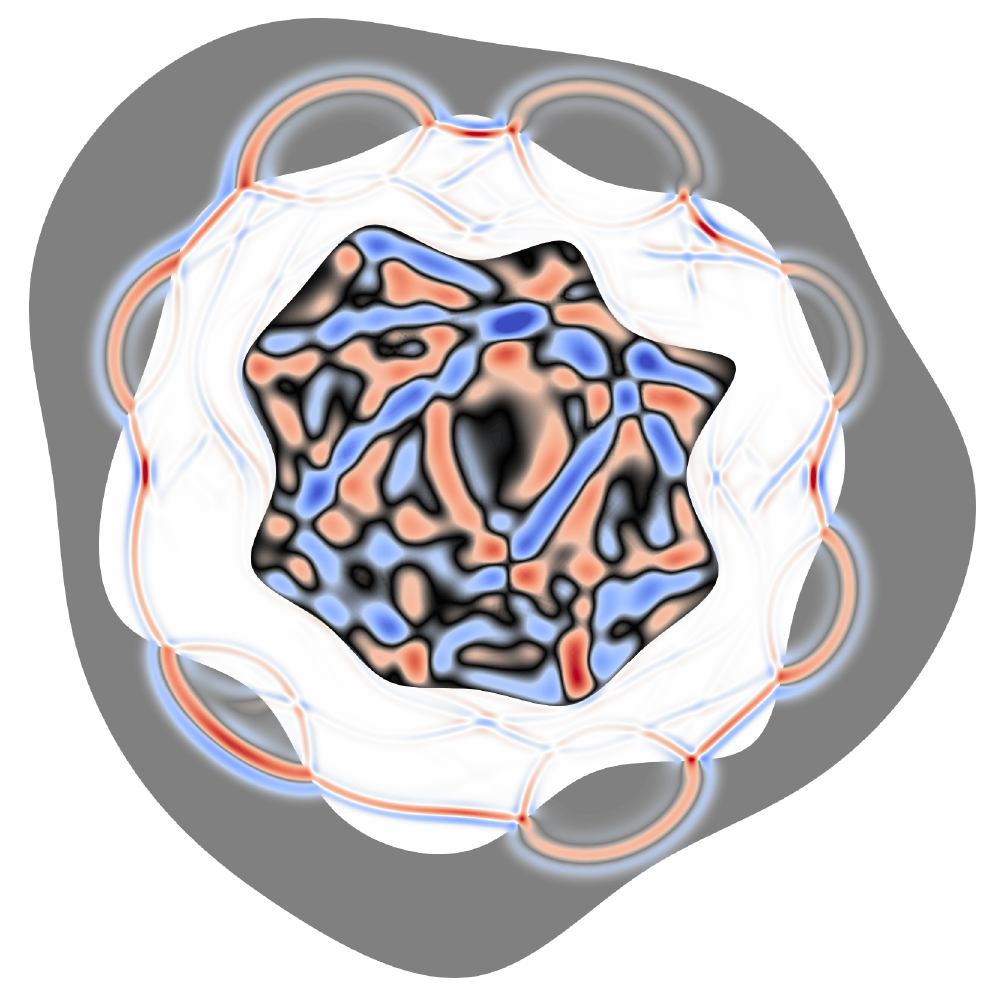
Here’s a simulation that shows what the ultrasound wavefield would look like when these waves would be transmitted into the brain:

The skull acts as a strong reflector of the ultrasound waves since the material contrast between soft tissue and bone is very large. This makes it tricky to get enough useful signal back from which we can create images of the brain.

This is exactly why this type of modelling is important. Since the signals we’re dealing with are so complicated, it’s important that we’re able to accurately model what’s going on when we try to propagate ultrasound waves into the brain so that we can extract as much information as possible out of the ultrasound signals we record.

---

Some Technical Details

There are a few main ingredients that make up the acoustic wave equation, namely:

Quantity	Meaning
\(\boldsymbol{x}\)	Location in space (\(x\)-, \(y\)-, and \(z\)-coordinates).
\(t\)	Time.
\(\rho (\boldsymbol{x})\)	Density of the material.
\(v_p (\boldsymbol{x})\)	Speed-of-sound in the material.
\(f (\boldsymbol{x}, t)\)	Source we are injecting at a particular location.
\(\varphi (\boldsymbol{x}, t)\)	Scalar potential; essentially the pressure within the material. This is what we’ll be solving for.

$$ \frac{1}{\rho v_p^2} \partial_t^2 \varphi - \nabla \cdot \left( \frac{1}{\rho} \nabla \varphi \right) = f. $$

There are certain “special cases” for which we can calculate a solution to the wave equation analytically (eg. for a simple homogeneous medium). If we think of most practical applications though, we’d normally want to have some more complicated (heterogeneous) material properties where \(v_p\) and/or \(\rho\) would vary throughout the medium. However, there’s unfortunately no feasible way to solve this equation analytically for cases where the material properties are heterogeneous. To get around this, we use numerical methods such as the finite-element or the finite-difference methods to approximate a solution of the wave equation.

In the above examples, we’ve used the solver Salvus (developed by Mondaic) which uses a special version of the finite-element method known as the spectral-element method. For more information on Salvus, see here.